Is The Ratio of Normal Variables Normal?

In Trustworthy Online Controller Experiments I came across this quote, referring to a ratio metric \(M = \\frac{X}{Y}\), which states that:

Because \(X\) and \(Y\) are jointly bivariate normal in the limit, \(M\), as the ratio of the two averages, is also normally distributed.

That’s only partially true. According to https://en.wikipedia.org/wiki/Ratio_distribution, the ratio of two uncorrelated noncentral normal variables \(X = N(\\mu\_X, \\sigma\_X^2)\) and \(Y = N(\\mu\_Y, \\sigma\_Y^2)\) has mean \(\\mu\_X / \\mu\_Y\) and variance approximately \(\\frac{\\mu\_X^2}{\\mu\_Y^2}\\left( \\frac{\\sigma\_X^2}{\\mu\_X^2} + \\frac{\\sigma\_Y^2}{\\mu\_Y^2} \\right)\). The article implies that this is true when \(Y\) is unlikely to assume negative values, say \(\\mu\_Y > 3 \\sigma\_Y\).

As always, the best way to believe something is to see it yourself. Let’s generate some uncorrelated normal variables far from 0 and their ratio:

ux = 100
sdx = 2
uy = 50
sdy = 0.5

X <- rnorm(1000, mean = ux, sd = sdx)
Y <- rnorm(1000, mean = uy, sd = sdy)
Z <- X / Y

Their ratio looks normal enough:

hist(Z)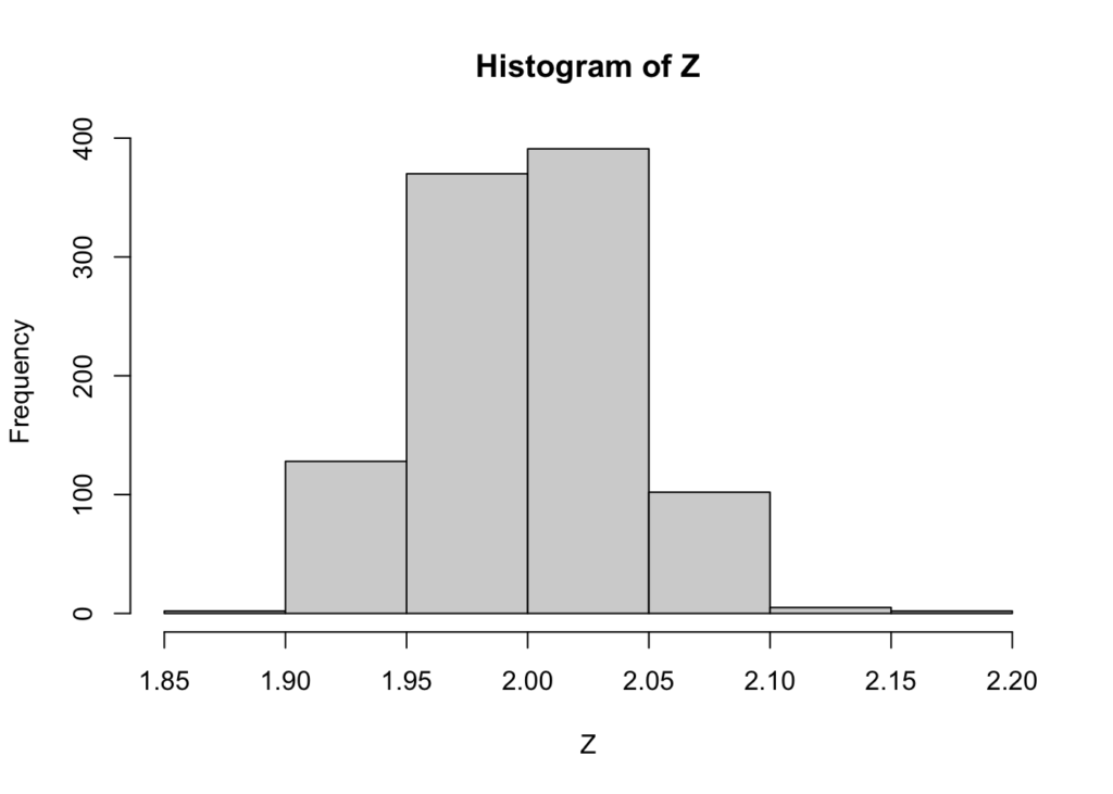

Which is confirmed by a q-q plot:

qqnorm(Z)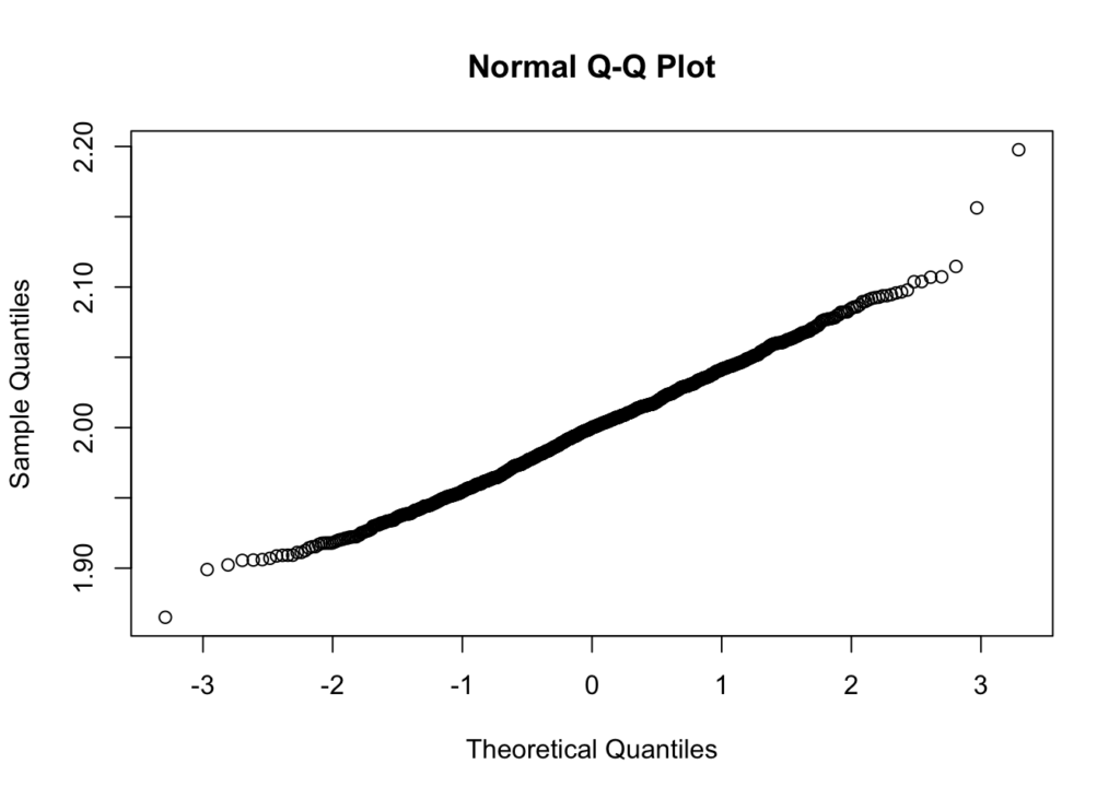

What about the mean and variance?

mean(Z)

[1] 1.998794

ux / uy

[1] 2

var(Z)

[1] 0.001783404

ux^2 / uy^2 * (sdx^2 / ux^2 + sdy^2 / uy^2)

[1] 0.002

Both the mean and variance are very close to their theoretical values.

But what happens now when the denominator \(Y\) has a mean close to 0?

ux = 100
sdx = 2
uy = 10
sdy = 2

X <- rnorm(1000, mean = ux, sd = sdx)
Y <- rnorm(1000, mean = uy, sd = sdy)
Z <- X / Y

Hard to call the resulting ratio normally distributed:

hist(Z)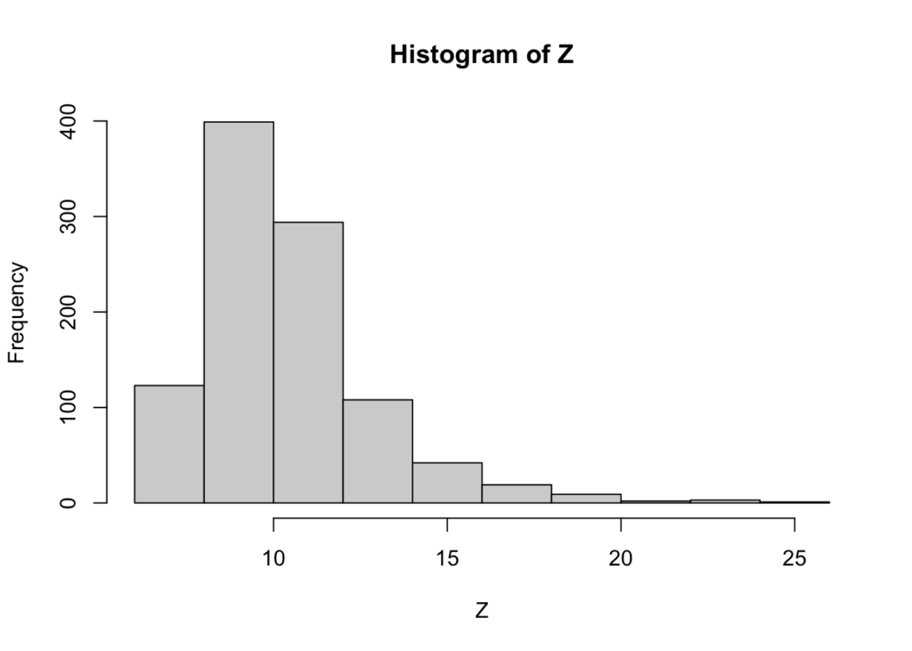

Which is also clear with a q-q plot:

qqnorm(Z)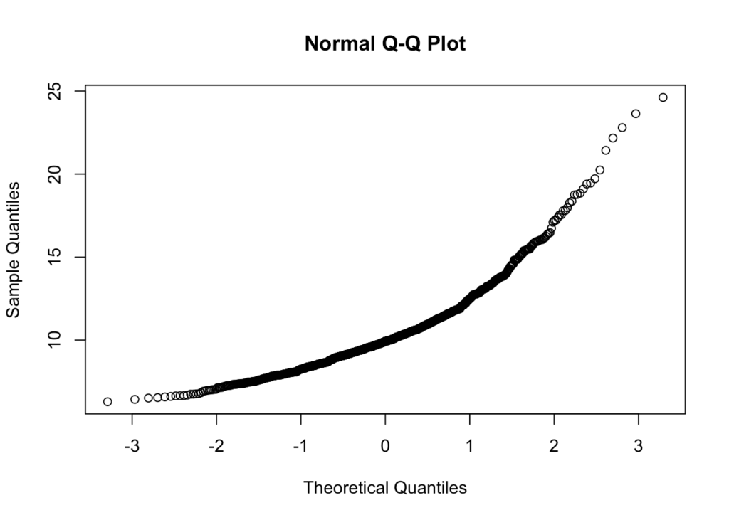

In other words, it is generally true that ratio metrics where the denominator is far from 0 will also be close enough to a normal distribution for practical purposes. But when the denominator’s mean is, say, closer than 5 sigmas from 0 that assumption breaks down.