Explore how the mean, median, and Hodges–Lehmann estimator tell different stories about treatment effects—and why the question should guide your choice.
r
statistics
Published
September 9, 2026
When I was studying physics we had our required share of lab work, which was also our introduction to experimental statistics. It was there that I heard for the first time about hypothesis testing, in particular about the t-test. And since I never formally studied statistics, I always assumed this test was one of the most fundamental ones. How wrong I was.
The problem with the t-test, which is often overlooked, lies in the assumptions it relies on—particularly the normality assumption. Violations of this assumption, we’re told, can introduce bias. This makes it sound as if the error is minor at worst; in fact it can lead to completely wrong conclusions.
Imagine we have an experiment with 300 pairs of matched subjects, where one member of each pair, chosen at random, gets some treatment. For each pair \(i\) we measure \(d_i = r_{Ti} - r_{Ci}\), the difference in responses between the treated unit and the control unit. Let’s assume that \(d_i\) isn’t normally distributed but instead follows a shifted lognormal distribution:
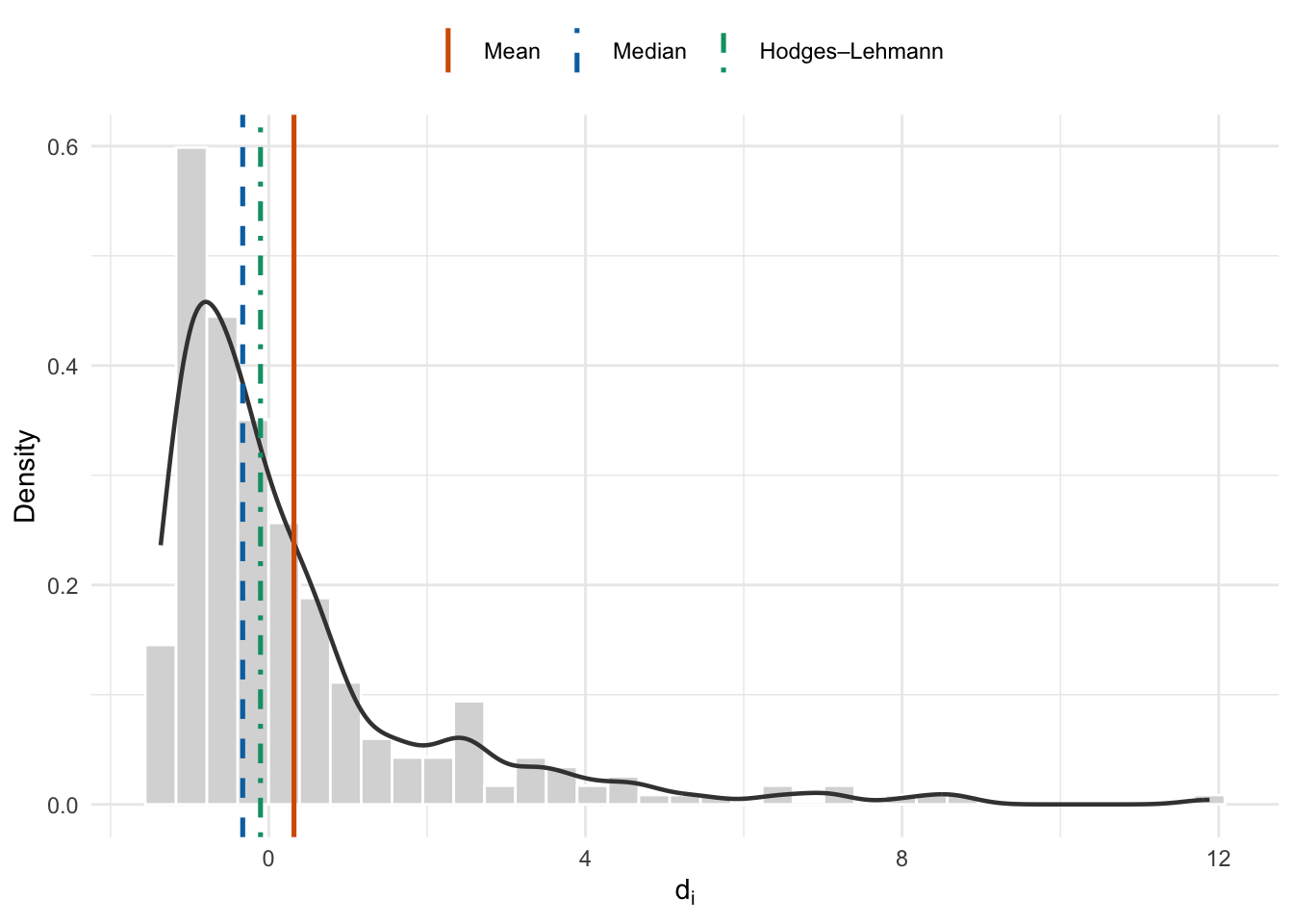
The plot above shows the histogram of this distribution and a density plot. As you’d expect from a lognormal distribution, there’s a heavy tail and the mean is substantially larger than the median. In fact, they are of opposite signs!
What is a point estimate anyway? It’s the value of an estimator. What do we want from an estimator? Whatever you want but people usually want it to be unbiased. Statistics 101 textbooks define a (usually) unbiased estimator as one that maximizes the likelihood. The likelihood of what? Of the model that you assume describes the distribution of the data. An equivalent definition is that it’s an unbiased estimator of the parameter you’re trying to estimate. What parameter? The parameter of the model that you assume describes the distribution of the data. What I’m saying is that by choosing an estimand—fancy name for the quantity you’re estimating—you’ve already committed to a model that you assumes describes the data you’ve collected.
Coming back to that lognormal distribution. In the plot above we show three reference lines:
the median: gives you the minimum effect size for half the population
Yeah, I know, this is not something you come across in introductory textbooks. Or job interviews for that matter. I learned about it from a textbook about observational studies, like, three weeks ago. Think of it as the appropriate point estimator when you’re using the non-parametric signed-rank test instead of the t-test. We don’t need to discuss how it’s defined; we just need to know that it is returned by the wilcox.test() function when setting conf.int = TRUE as the estimate value of the returned list.
The HL estimator is, strictly speaking, only useful when the distribution is symmetric. Like the mean or the median it is a location estimator. It is robust against outliers (unlike the mean) but more reliable than the median. Use it for “serious” decisions like launch decisions, but stick to the median in stakeholder presentations.
It bears repeating: which estimator to use depends on the application. You want to use the mean if you worry about the average impact of your treatment; you want to use the median or the HL estimator if you worry about the impact on the middle customer experience. This is a product decision, not a data science one.
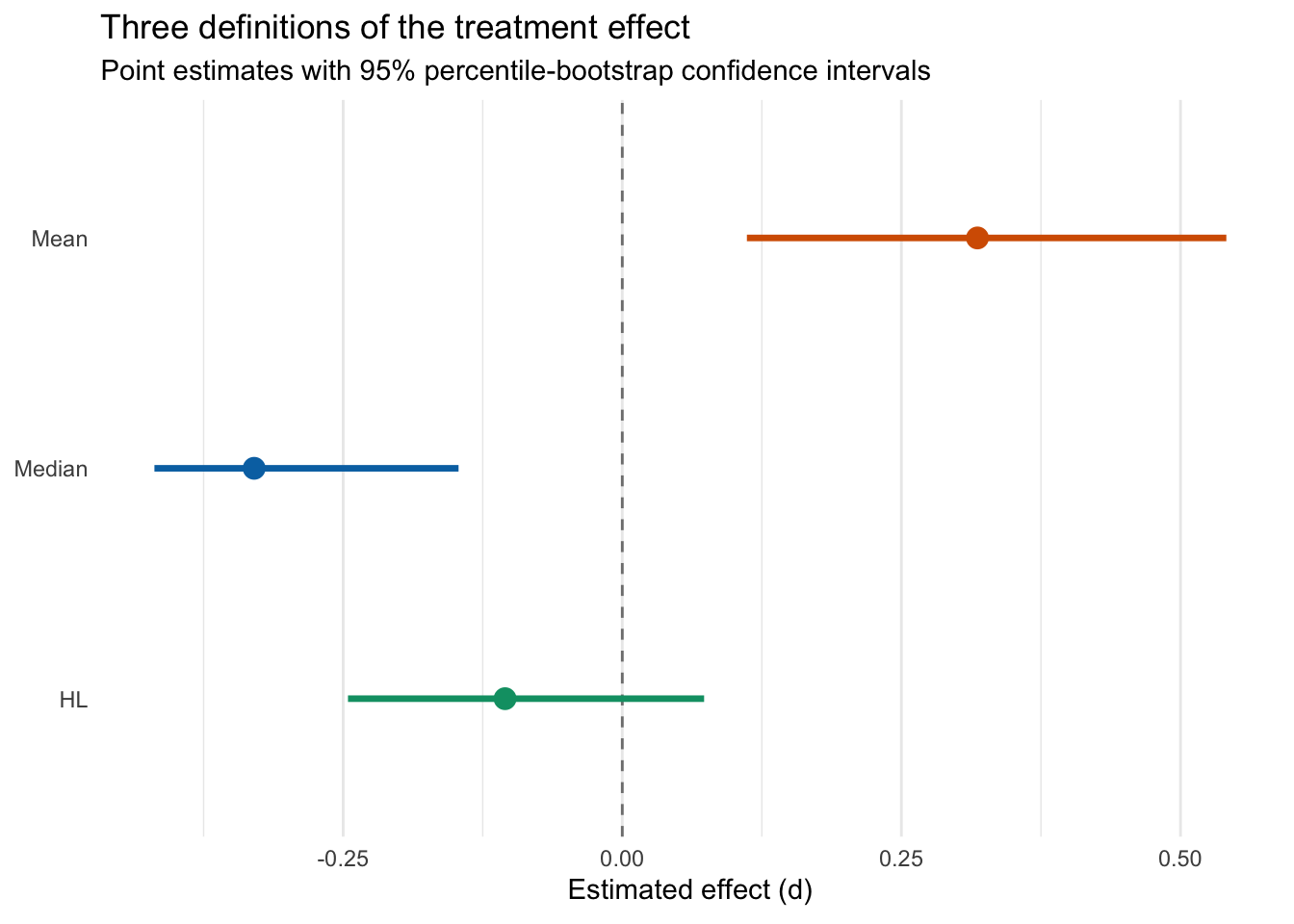
On a final note, for these estimators we can bootstrap the matched-pair differences to estimate their confidence intervals:
  estimand   estimate   lower_95    upper_95
1     Mean  0.3181297  0.1116221  0.54105203
2   Median -0.3297339 -0.4190513 -0.14664311
3       HL -0.1049871 -0.2456868  0.07329634
This shows that the percentile-bootstrap intervals for the median and HL estimator are both narrower than the mean’s interval:
Taken together, these results underscore why the estimand must follow the business question. The mean, median, and HL estimator all tell a completely different story because they describe different aspects of the same data, and can therefore support different decisions. Choosing the relevant quantity requires business judgment; estimating it correctly requires statistical judgment. Good data science needs both.