Why can both X / Y and Y / X average more than 1?

In an earlier post I explored under what assumptions the ratio of normal variables could be approximately normal. In our simulations, when the means were large compared to the standard deviations, the sample average of the ratio was close to the ratio of the sample means. There is a subtle distinction here between a sample average and a population expectation, which we’ll come back to.

Things get awkward when the denominator can get close to zero and the ratio can blow up. But here is an even more counterintuitive result: for two independent, identically distributed positive random variables \(X\) and \(Y\), both \(X/Y\) and \(Y/X\) can have an expected value \(> 1\).

(The equality is less surprising: because \(X\) and \(Y\) are independent and identically distributed, swapping them leaves their joint distribution unchanged. So \(X/Y\) and \(Y/X\) have the same distribution, and the same expectation whenever it exists. The puzzle is why that expectation can exceed 1.)

This matters when summarizing paired measurements, such as right and left foot lengths. Averaging individual ratios estimates a different quantity from taking the ratio of the population means. Neither is inherently wrong, but interpreting the former as relative lift defined by the latter can be misleading. Paired measurements may also be correlated; the simulation below isolates the effect using independent draws.

Let’s see the effect in action with some simulations. We’re going to draw independent values of \(X\) and \(Y\), each normally distributed with mean 1 and standard deviation 0.2, and look at both ratios:

set.seed(20260924)
n <- 1000000
mu <- 1
sigma <- 0.2
X <- rnorm(n, mean = mu, sd = sigma)
Y <- rnorm(n, mean = mu, sd = sigma)

summarize_ratios <- function(x, y) {
  data.frame(
    pairs = length(x),
    mean_X = mean(x),
    mean_Y = mean(y),
    ratio_of_means = mean(x) / mean(y),
    mean_X_over_Y = mean(x / y),
    mean_Y_over_X = mean(y / x)
  )
}

knitr::kable(summarize_ratios(X, Y), digits = 4)

pairs	mean_X	mean_Y	ratio_of_means	mean_X_over_Y	mean_Y_over_X
1e+06	0.9999	1	0.9999	1.0461	1.0463

Both sample averages of ratios are above 1, although the ratio of sample means is close to 1.

(There is one technical catch: for independent, untruncated normals, the population ratio mean is undefined, even when the sample average looks stable.¹ To talk about expectations, we’ll keep both variables within four standard deviations of their mean: between 0.2 and 1.8. The resulting truncated normals remain independent, with population means exactly 1 by symmetry.)

lower <- 0.2
upper <- 2 * mu - lower
keep <- X >= lower & X <= upper & Y >= lower & Y <= upper
x <- X[keep]
y <- Y[keep]

knitr::kable(summarize_ratios(x, y), digits = 4)

pairs	mean_X	mean_Y	ratio_of_means	mean_X_over_Y	mean_Y_over_X
999870	0.9999	1	0.9999	1.0459	1.0462

This removes just 130 of our 1,000,000 pairs, and both ratio averages are still above 1.

So what’s going on here? This is where Jensen’s inequality comes in. It’s probably the coolest inequality you’ve never heard of, and it says that for a convex function \(f\), \(E[f(Y)] \geq f(E[Y])\). That felt abstract to me until I noticed that the reciprocal function \(f(y)=1/y\) is strictly convex for \(y>0\), and this is why downward fluctuations of a denominator (like \(Y\) in \(X/Y\)) increase the reciprocal more than equally sized upward fluctuations decrease it.

We can see this directly in our simulated denominators. Average them first and then take the reciprocal: 1 / mean(y) is 1.0000. Take each reciprocal first and then average: mean(1 / y) is 1.0460. The same observations give different answers depending on the order of operations. Since the independent numerator has population mean 1, this increase carries over to the expected ratio.

For our truncated variables, independence and strict convexity give

\[ \begin{aligned} E[X/Y] &= E[X]E[1/Y] > \frac{E[X]}{E[Y]} = 1, \\ E[Y/X] &= E[Y]E[1/X] > \frac{E[Y]}{E[X]} = 1. \end{aligned} \]

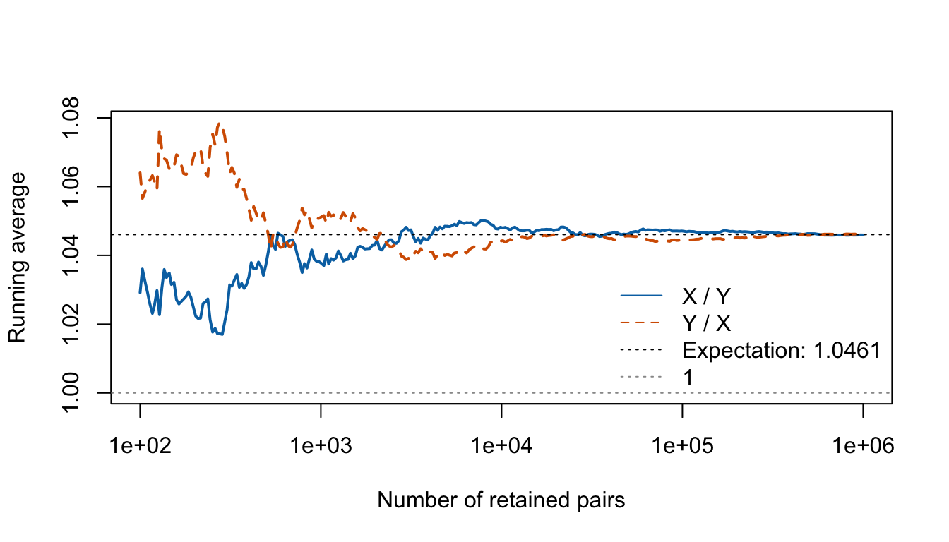
The inequality is strict because each denominator varies. Since \(X\) and \(Y\) have the same distribution, the two expectations are equal. Let’s compare their running averages with the common expectation, calculated by numerical integration.

mass <- pnorm(upper, mu, sigma) - pnorm(lower, mu, sigma)
expected_ratio <- mu * integrate(
  function(z) dnorm(z, mu, sigma) / (z * mass),
  lower = lower, upper = upper
)$value

k <- unique(round(exp(seq(log(100), log(length(x)), length.out = 300))))
running <- cbind(cumsum(x / y)[k] / k, cumsum(y / x)[k] / k)
matplot(
  k, running, type = "l", log = "x", lty = c(1, 2),
  col = c("#0072B2", "#D55E00"), lwd = 2,
  ylim = range(1, expected_ratio, running),
  xlab = "Number of retained pairs", ylab = "Running average"
)
abline(h = 1, col = "grey60", lty = 3)
abline(h = expected_ratio, col = "black", lty = 3)
legend(
  "bottomright",
  legend = c("X / Y", "Y / X", sprintf("Expectation: %.4f", expected_ratio), "1"),
  col = c("#0072B2", "#D55E00", "black", "grey60"),
  lty = c(1, 2, 3, 3), bty = "n"
)

Figure 1: Both running averages approach the same expectation above 1 for the truncated normals.

The simulation agrees with the theory: for these independent truncated normals, both sample averages approach the same expectation, about 1.0461. Each pair of ratios multiplies to 1, but their averages need not. Averaging and taking reciprocals are different operations—and Jensen’s inequality tells us which way the difference goes.

Footnotes

1. This corrects the earlier post’s claim about the population mean. A normal variable equals zero with probability zero, but its density stays positive arbitrarily close to zero. Consequently, the integral defining \(E[|1/Y|]\) diverges like \(\int_0^\epsilon dy/y\), and the positive and negative parts of the ratio’s expectation both diverge. See Yang and Gui. Keeping only positive values would still leave an infinite reciprocal mean; a strictly positive lower bound avoids the problem. The upper bound preserves symmetry about 1.